Climate Change Explorer V1.0
Welcome to the GYA Climate Explorer
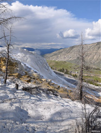
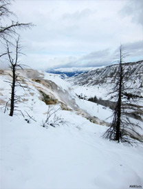
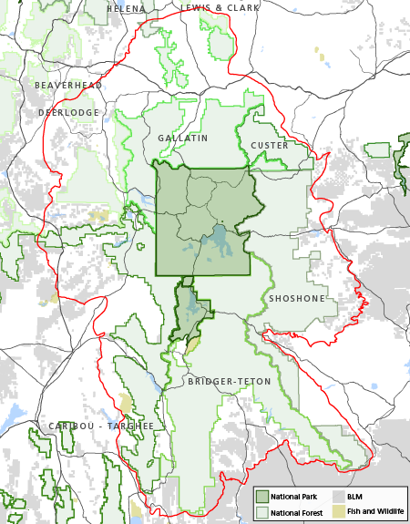
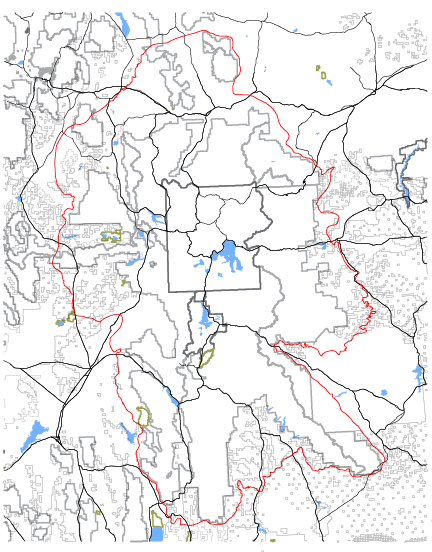
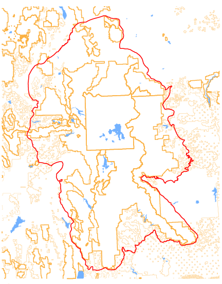
The goal of this project is to examine climate change data for the Greater Yellowstone Area (GYA). For each variable on the right-hand toolbar, the GYA Climate Explorer compares the average of historic (1916 - 2006) climate values to a future projection for the mid-century (Ensemble Mean 2030 - 2059 values). There are three graphical representations of the data: stacked historic and mid-century maps with a slider bar to compare pixel values between the two, a delta map showing change for each pixel value, and a bar graph or pie chart showing a comparison of the historic and mid-century values. The graphs represent data from the Ecoshare website that has been clipped to the GYA extent shown as a red polygon on the map above. More information can be found on the "About" page. Explore the site and contact us with questions!
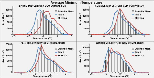
Spring (MAM) Average Minimum Temperature

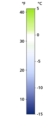

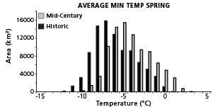
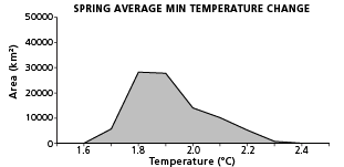

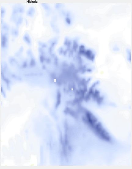

Springtime (MAM) minimum temperatures (daily low) are projected to warm by 2.9 to 4.1°F (1.6 to 2.3°C) by the middle of this century (2030-2059). This projection is the average of 10 global climate models using the IPCC’s A1B emissions scenario. A1B is a middle-level scenario for both carbon dioxide emissions and economic growth, with carbon dioxide levels rising from 390 ppmv at present to 550 ppvm by the mid-2050s.
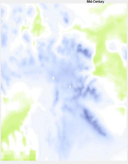
Summer (JJA) Average Minimum Temperature
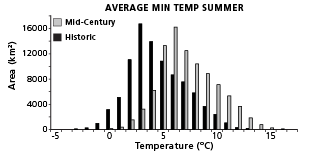
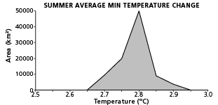
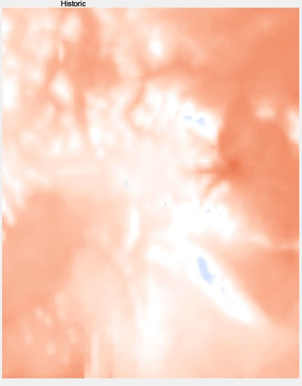
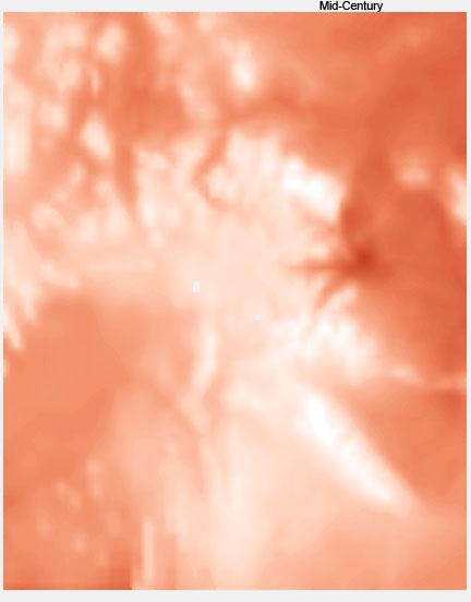

Summer (JJA) minimum temperatures (daily low) are projected to warm by 4.7 to 5.3°F (2.65 to 2.95°C) by the middle of this century (2030-2059). This projection is the average of 10 global climate models using the IPCC’s A1B emissions scenario. A1B is a middle-level scenario for both carbon dioxide emissions and economic growth, with carbon dioxide levels rising from 390 ppmv at present to 550 ppvm by the mid-2050s.
Fall (SON) Average Minimum Temperature
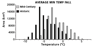
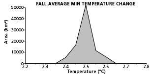
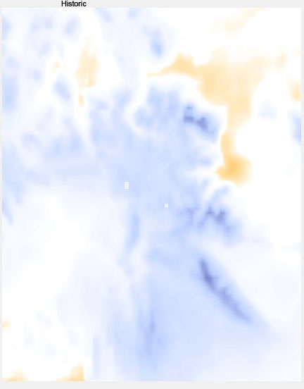
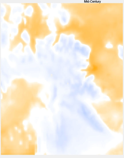

Autumn (SON) minimum temperatures (daily low) are projected to warm by 4.2 to 4.8°F (2.35 to 2.65°C) by the middle of this century (2030-2059). This projection is the average of 10 global climate models using the IPCC’s A1B emissions scenario. A1B is a middle-level scenario for both carbon dioxide emissions and economic growth, with carbon dioxide levels rising from 390 ppmv at present to 550 ppvm by the mid-2050s.
Winter (DJF) Average Minimum Temperature
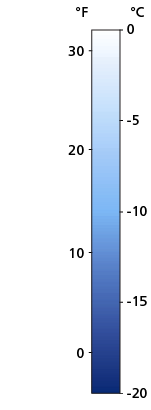
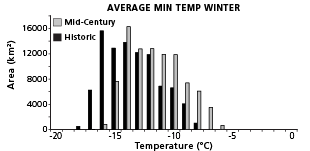
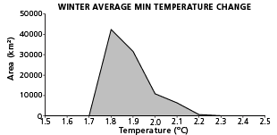
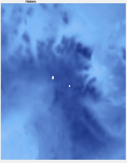

Winter (DJF) minimum temperatures (daily low) are projected to warm by 3.1 to 4.1°F (1.7 to 2.3°C) by the middle of this century (2030-2059). This projection is the average of 10 global climate models using the IPCC’s A1B emissions scenario. A1B is a middle-level scenario for both carbon dioxide emissions and economic growth, with carbon dioxide levels rising from 390 ppmv at present to 550 ppvm by the mid-2050s.
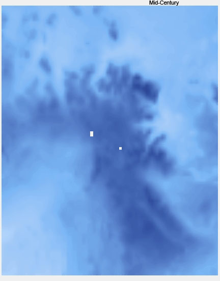
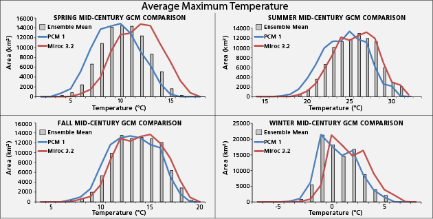
Summer (JJA) Average Maximum Temperature
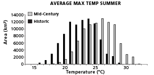
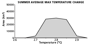
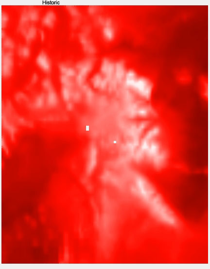
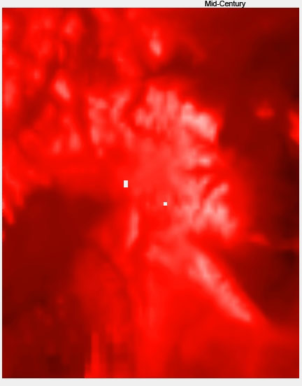

Summer (JJA) maximum temperatures (daily high) are projected to warm by 4.8 to 5.3°F (2.55 to 2.95°C) by the middle of this century (2030-2059). This projection is the average of 10 global climate models using the IPCC’s A1B emissions scenario. A1B is a middle-level scenario for both carbon dioxide emissions and economic growth, with carbon dioxide levels rising from 390 ppmv at present to 550 ppvm by the mid-2050s.
Spring (MAM) Average Maximum Temperature
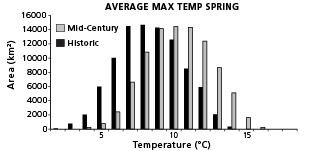

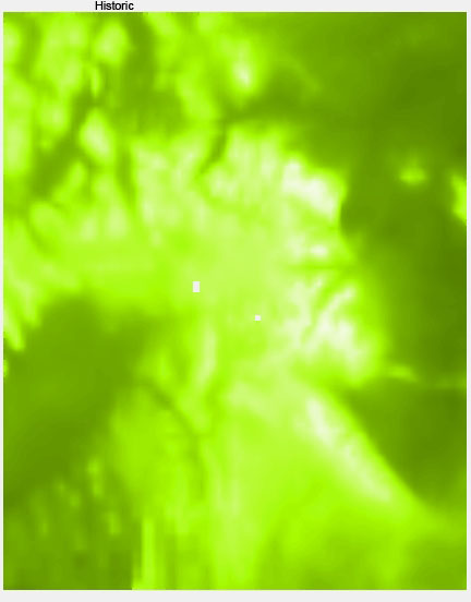
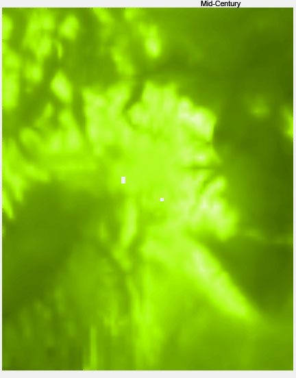

Springtime (MAM) maximum temperatures (daily high) are projected to warm by 2.9 to 4.1°F (1.6 to 2.3°C) by the middle of this century (2030-2059). This projection is the average of 10 global climate models using the IPCC’s A1B emissions scenario. A1B is a middle-level scenario for both carbon dioxide emissions and economic growth, with carbon dioxide levels rising from 390 ppmv at present to 550 ppvm by the mid-2050s.
Fall (SON) Average Maximum Temperature
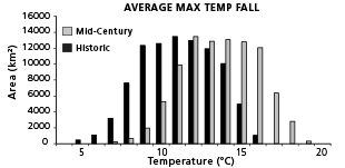
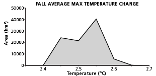
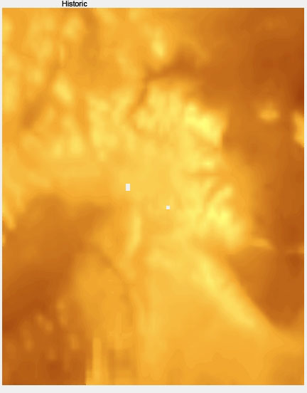
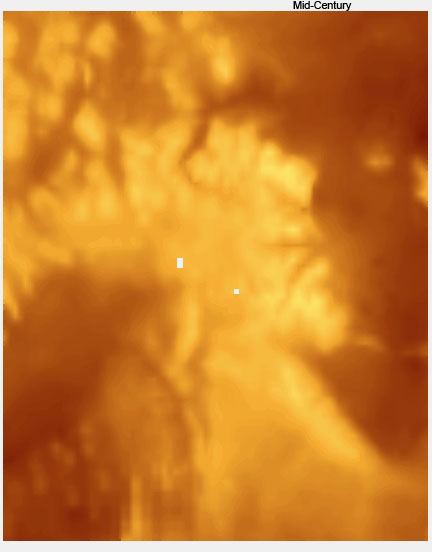

Fall (SON) maximum temperatures (daily high) are projected to warm by 4.3 to 4.8°F (2.4 to 2.7°C) by the middle of this century (2030-2059). This projection is the average of 10 global climate models using the IPCC’s A1B emissions scenario. A1B is a middle-level scenario for both carbon dioxide emissions and economic growth, with carbon dioxide levels rising from 390 ppmv at present to 550 ppvm by the mid-2050s.
Winter (DJF) Average Maximum Temperature
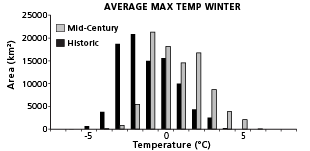
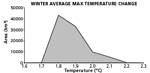
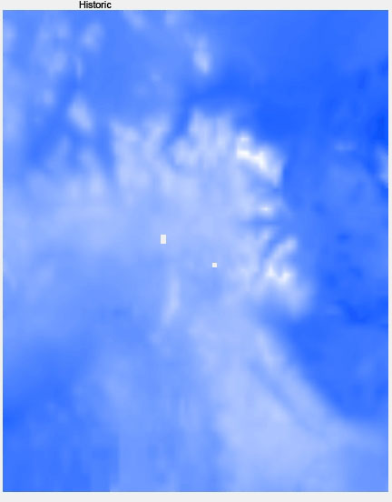

Winter (DJF) maximum temperatures (daily high) are projected to warm by 3.1 to 4.1°F (1.7 to 2.3°C) by the middle of this century (2030-2059). This projection is the average of 10 global climate models using the IPCC’s A1B emissions scenario. A1B is a middle-level scenario for both carbon dioxide emissions and economic growth, with carbon dioxide levels rising from 390 ppmv at present to 550 ppvm by the mid-2050s.
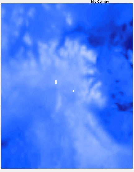
Spring (MAM) Average Temperature
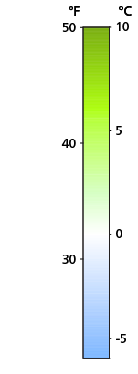
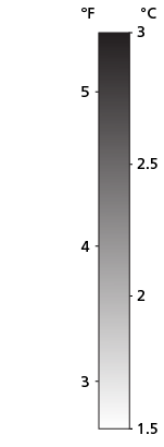
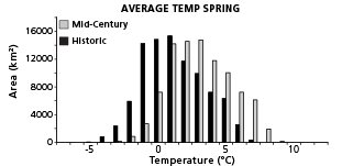
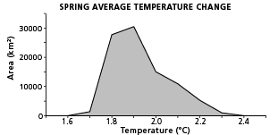
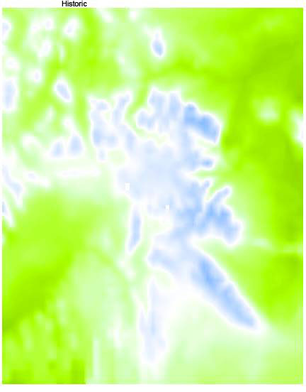
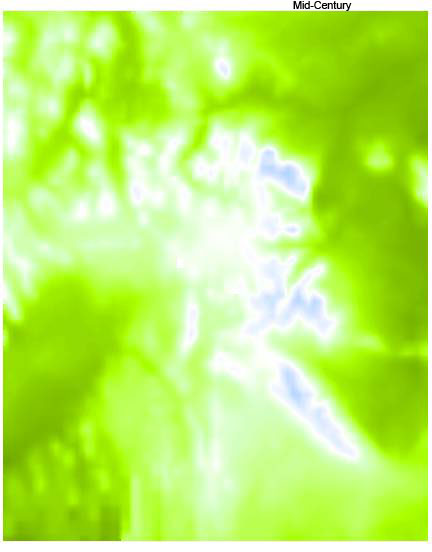

Springtime (MAM) average temperatures in the Greater Yellowstone Area are projected to warm by 2.9° to 4.3°F (1.6 to 2.4°C) by the middle of the 21st century (2030-2059) compared to the average from 1970-1999. This projection is the average of 10 global climate models using the IPCC’s A1B emissions scenario. A1B is the middle-level scenario for both carbon dioxide emissions and economic growth, with atmospheric concentrations of CO2 rising from 390 ppmv at present to 550 ppvm by mid-century.
Summer (JJA) Average Temperature
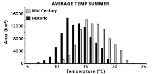
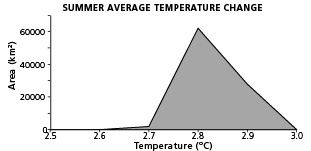
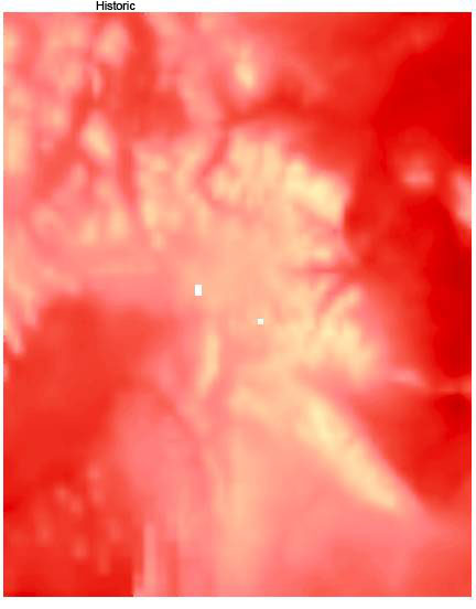
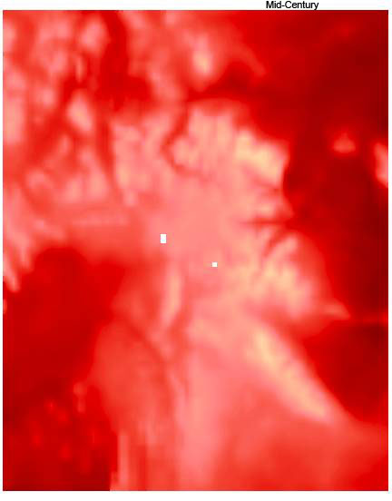

Summer (JJA) average temperatures in the Greater Yellowstone Area are projected to warm by 4.7° to 5.4°F (2.6 to 3.0°C) by the middle of the 21st century (2030-2059). Summer average temperatures are projected to warm more than other seasons. This projection is the average of 10 global climate models using the IPCC’s A1B emissions scenario. A1B is the middle-level scenario for both carbon dioxide emissions and economic growth, with atmospheric concentrations of CO2 rising from 390 ppmv at present to 550 ppvm by mid-century.
Fall (SON) Average Temperature
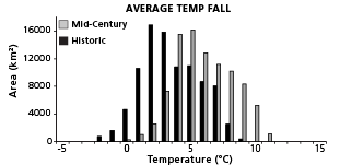
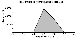
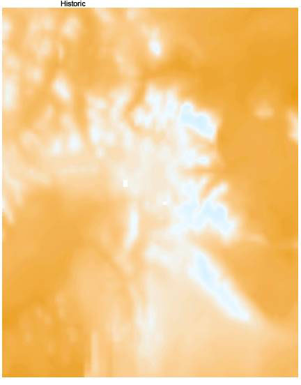

Fall (SON) average temperatures in the Greater Yellowstone Area are projected to warm by 4.3° to 4.9°F (2.3 to 2.7°C) by the middle of the 21st century (2030-2059). This projection is the average of 10 global climate models using the IPCC’s A1B emissions scenario. A1B is the middle-level scenario for both carbon dioxide emissions and economic growth, with atmospheric concentrations of CO2 rising from 390 ppmv at present to 550 ppvm by mid-century.
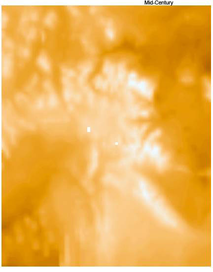
Winter (DJF) Average Temperature
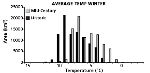
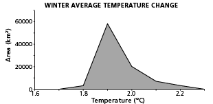


Winter (DJF) average temperatures in the Greater Yellowstone Area are projected to warm by 3.1° to 4.1°F (1.7 to 2.3°C) by the middle of the 21st century (2030-2059). This projection is the average of 10 global climate models using the IPCC’s A1B emissions scenario. A1B is the middle-level scenario for both carbon dioxide emissions and economic growth, with atmospheric concentrations of CO2 rising from 390 ppmv at present to 550 ppvm by mid-century.
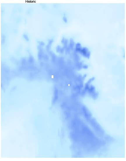
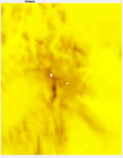
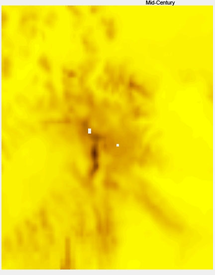
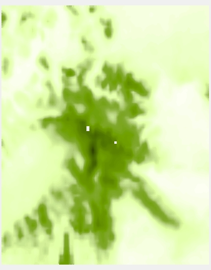
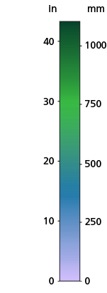
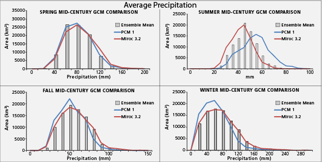
Spring (MAM) Average Precipitation
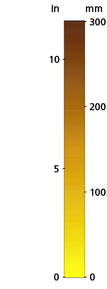
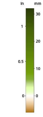
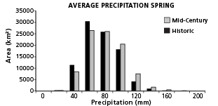
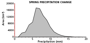
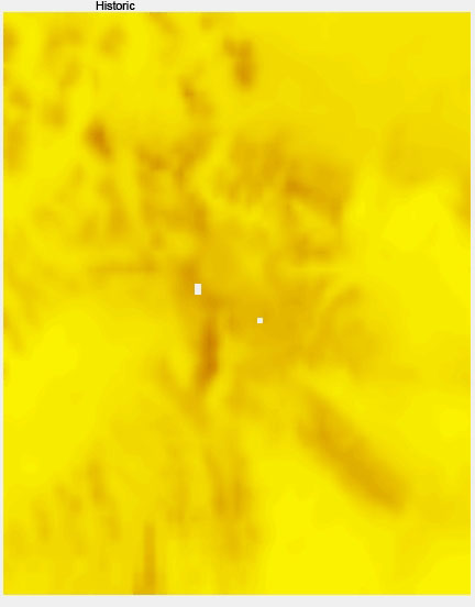
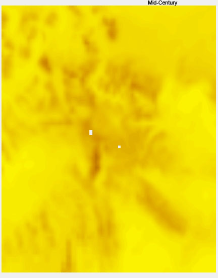
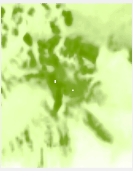
Springtime mean precipitation is projected to increase by 0.04 to 0.6 inches (2.54 to 15.24 mm) by the mid-21st century (2030-2059), with the largest increases over areas of relatively high elevations.
Summer (JJA) Average Precipitation
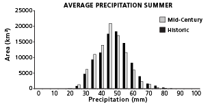
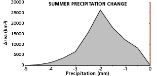
Summer precipitation is projected to decrease between 0.0 and 0.18 inches (0.0 to 4.57 mm) by the mid-21st century (2030-2059), with the larger decreases in the southern and western portions of the Greater Yellowstone area.
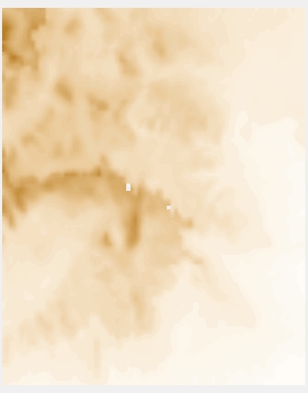
Fall (SON) Average Precipitation
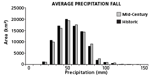
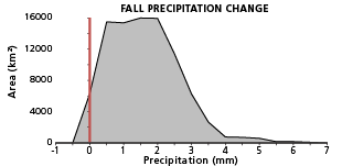
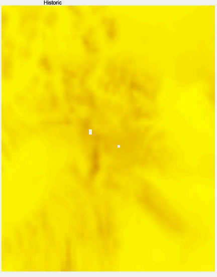
Autumn precipitation is projected to change by -0.04 to +0.24 inches (-1.0 to +6.1 mm) by the middle of this century (2030-2058), with the larger increases in the southwestern portion of the Greater Yellowstone area.
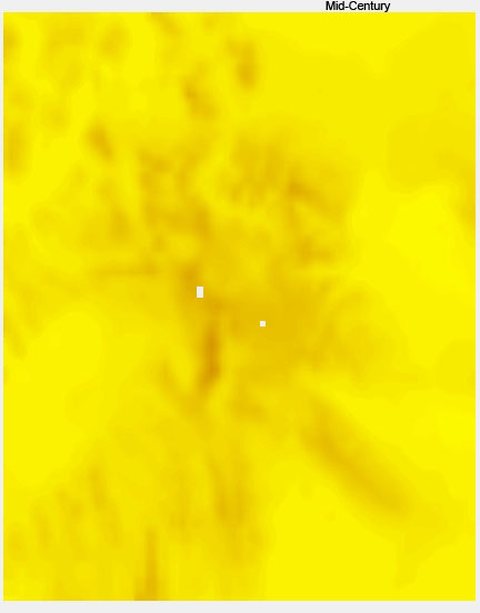
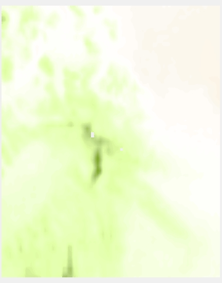
Winter (DJF) Average Precipitation
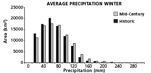
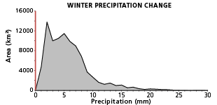
Winter precipitation is projected to increase from 0.0 to 0.94 inches (0.0 to 23.9 mm) by the middle of this century, with the largest increases occurring over relatively high elevations of the GYA.
Spring (MAM) Combined Flow
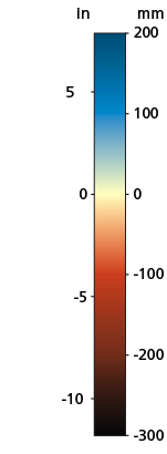
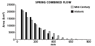
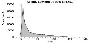
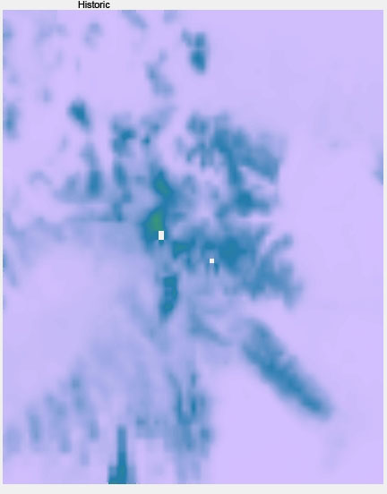
Combined (runoff plus baseflow) spring streamflow is projected to increase by 0.0 to 5.9 inches (0 to 149.86 mm). Areas of higher elevations are projected to see larger relative increases in spring combined flow.
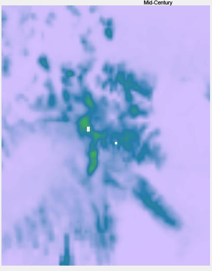
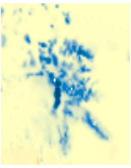
Summer (JJA) Combined Flow
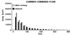
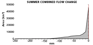
Summer combined flow is projected to decrease by 0.0 to 5.1 inches (0 to 129.54 mm) with larger decreases in areas of high elevations.
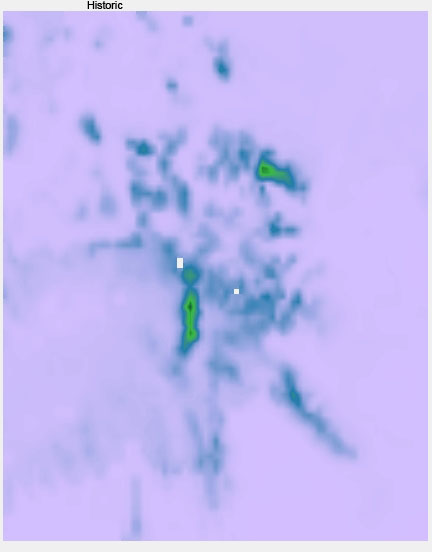
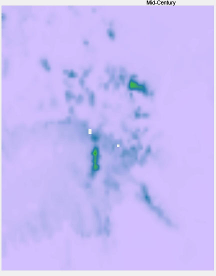
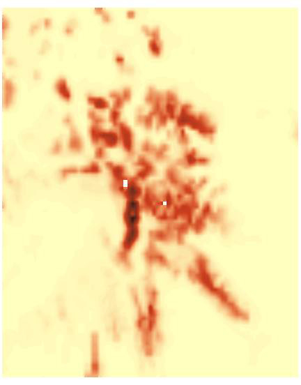
Fall (SON) Combined Flow
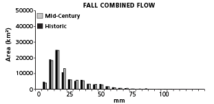
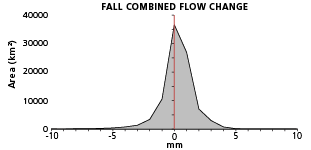


Autumn combined flow is projected to see relatively little change by the middle of this century, with the average of 10 models estimating a range of -0.2 to +0.2 inches (-5.08 to 5.08 mm).
Winter (DJF) Combined Flow
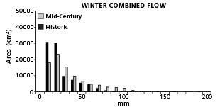
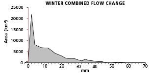

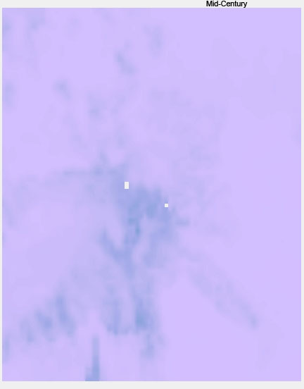
Combined flow in winter is projected to increase by 0.0 to 2.7 inches (0.0 to 68.37 mm), with the larger increases occurring over higher elevations.
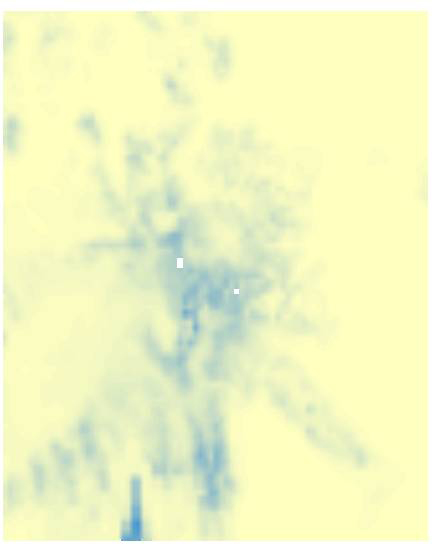
April Snow Water Equivalent (SWE)
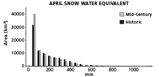
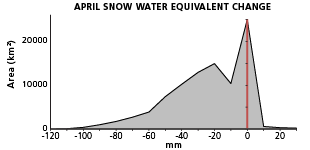
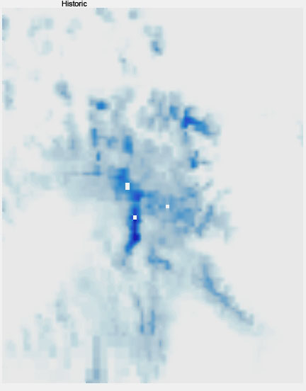
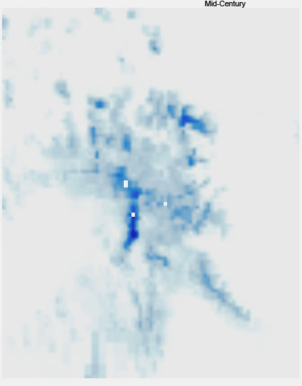
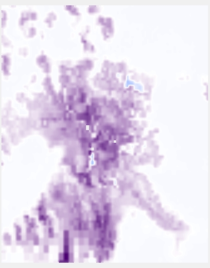
April 1 Snow Water Equivalent (SWE) is projected to change from +0.4 to -3.9 inches (10.16 to -99.06 mm), with the greatest declines in mid- to high elevations.
Snowpack Vulnerability
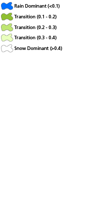
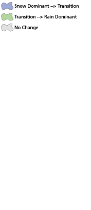
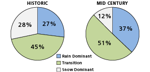

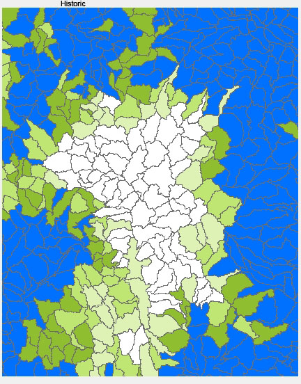
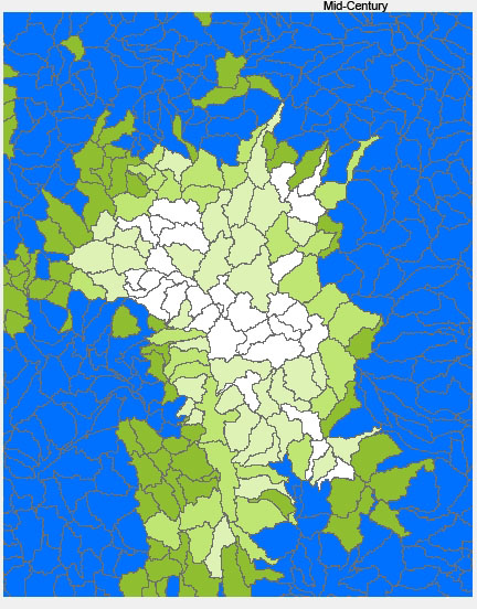
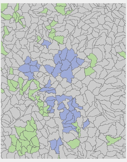
Snowpack vulnerability illustrates how much of the winter precipitation remains stored in spring snowpack. Technically, it is the ratio of April 1 SWE to cool season (ONDJFM) precipitation. “Snow dominated” watersheds are those with greater than 40% of winter precipitation stored in April 1 snowpack, “transitional” watersheds are those with between 10% and 40% of their winter precipitation stored in April 1 snowpack, and “Rain dominated” watersheds are those with >10% of their winter precipitation entrained in April 1 snowpack. By the middle of this century, 28 watersheds currently classified as snow dominant are expected to remain snow dominant. 56% (36 out of 64) of watershed currently classified as snow dominant watersheds in the GYA are likely to convert to transitional watersheds. 22% (22 out of 101) percent of watershed currently considered transitional are likely to change to rain dominant.
Global Climate Models Future climate projections rely on Global Climate Models (GCMs). A Global Climate Model is a numerical representation of the climate system based on the physical, chemical and biological properties of its components, their interactions, and feedback process. In 2007 the Intergovernmental Panel on Climate Change (IPCC) reviewed 23 different GCMs, each driven by a common set of greenhouse gas emission scenarios. Because GCMs are designed to evaluate the behavior of the global climate system, their spatial resolution is coarse, with grid cell sizes typically ranging from 150 km2 to 250 km2. As a result, GCMs generally do not capture finer-scale climatic and meteorological process, such as orographic precipitation, or fine-scale climatic variability. "Downscaling" GCM climate projections increases the spatial resolution of climate information allowing users to better visualize what these future climates may imply locally and regionally. The University of Washington's Climate Impact Group (CIG) downscaled data for the western U.S. from 10 GCMs, chosen by the CIG because they performed the best in the Northern Rockies/Upper Missouri and Central Rockies/Upper Colorado areas in simulating historic observed temperature and precipitation trends of the 20th century. Each of the 10 GCMs are driven by the A1B emissions scenario, which is a mid-level scenario for both carbon dioxide emissions and economic growth, with atmospheric concentrations of carbon dioxide rising from 390 ppmv (parts per million by volume) at present to 550 ppvm by the mid-2050s. These coarse climate projections were downscaled to a 1/16th degree latitude/longitude grid (~6 x 6 km) over most of the western U.S. using a modified Delta method. CIG applied the downscaled climate change projections to produce projections of hydrologic changes using the Variable Infiltration Capacity (VIC) model. Additional details on these methods can be found in Littell et al., 2011. The data used for the GYA Climate Explorer come from the downscaled GCM and VIC model simulations produced by CIG. The values from the 10 models have been combined and averaged into an ensemble mean that reduces bias from individual models. Variables The Ecoshare website provides ensemble mean GCM data for 16 variables. So far we have chosen six of those variables plus snowpack vulnerability for the GYA Climate Explorer. For each variable, the GYA Climate Explorer compares the average of historic (1916 - 2006) climate values to a future projection for the mid-century (Ensemble Mean 2030 - 2059 values).
| GYA CLIMATE EXPLORER VARIABLES | ADDITIONAL VARIABLES ON ECOSHARE |
|---|---|
| Minimum Temperature | PET 1 |
| Maximum Temperature | PET 5 |
| Average Temperature | Runoff |
| Precipitation | Snow Depth |
| Combined Flow | Relative Humidity |
| Snow Water Equivalent | Soil Moisture Deficit |
| Snowpack Vulnerability | Water Balance Deficit |
| Base Flow | |
| Evapotranspiration | |
| Soil Moisture |
Glossary
Emissions Scenario - A plausible representation of the future emissions of radiatively-active substances in the atmosphere, like greenhouse gases and aerosols. These scenarios are based on coherent and internally consistent assumptions about driving forces such as demographic and socioeconomic development, technological change, etc. To date, the IPCC has developed two sets of emissions scenarios: the IS92, used for the Second Assessment, and the SRES scenarios used for the TAR and AR4. GCM-based climate simulations for the AR5 will be based on "representative concentration pathways" (RCPs). Trajectories of emissions concentrations will drive the models without regard to the societal and natural forces that result in those emissions. In parallel, scenarios will be developed to see what socioeconomic development paths result in emissions concentrations corresponding to RCPs.
Generation Circulation Model - A numerical representation of the climate system based on the physical, chemical, and biological properties of its components, their interactions and feedback processes, and accounting for all or some of its known properties. The climate system can be represented by models of varying complexity (ie, for any one component or combination of components a hierarchy of models can be identified, differing in such aspects as the number of spatial dimensions, the extent to which physical, chemical, or biological processes are explicitly represented, or the level at which empirical parameterisations are involved. Coupled atmosphere/ ocean/sea-ice General Circulation Models (AOGCMs) provide a comprehensive representation of the climate system. More complex models include active chemistry and biology. Climate models are applied, as a research tool, to study and simulate the climate, but also for operational purposes, including monthly, seasonal, and interannual climate predictions.
Ecoshare Variables
Average Temperature - This is the average temperature in degree Celsius for the month, season or year for the time period. For example, an average temperature for "Jan" would be an average of the high and low temperatures for every day in January for each year in the time period.
Base Flow - This is the portion of the stream-flow that would be present even during periods of drought. Monthly and seasonal totals averaged over various time periods are available (in mm).
Combined Flow - This is base flow plus runoff. Monthly and seasonal totals averaged over various time periods are available (in mm).
Evapotranspiration - This is the loss of water to the atmosphere as a result of evaporation and the transpiration of plants measured in mm. Summer monthly and seasonal totals averaged over various time periods are available.
Maximum Temperature - Average daily maximum temperature in degrees Celsius aggregated by months. This is the average of the daily maximum temperatures. For example, a maximum temperature for "Jan" would be an average of the high temperatures for every day in January for each year in the time period.
Minimum Temperature - Average daily minimum temperature in degrees Celsius aggregated by months. This is the average of the daily minimum temperatures. For example, a minimum temperature for "Jan" would be an average of the low temperatures for every day in January for each year in the time period.
PET1 - This is the potential evapotranspiration for natural vegetation, no water limit. Summer monthly and seasonal totals averaged over various time periods are available (in mm).
PET5 - This is the potential evapotranspiration for a short reference crop (short grass). Summer monthly and seasonal totals averaged over various time periods are available (in mm).
Precipitation - Monthly average precipitation amount in mm. This is the monthly and annual totals averaged over various time periods, and monthly totals averaged over seasons and various time periods. For example, precipitation for "Jan" would be an average of the rainfall or snow water equivalent for the entire month for each January in the time period; precipitation for winter would be the average monthly precipitation for every December, January and February in the time period.
Relative Humidity - This is the ratio of the amount of moisture actually in the air to the maximum amount of moisture which the air could hold at the same temperature, expressed as a percent. Summer monthly and seasonal averages are available.
Runoff - This is the water, measured in mm, that moves across the surface, or just beneath the surface, coming from precipitation or the melting of ice and snow. Monthly and seasonal totals averaged over various time periods are available.
Soil Moisture - This is the portion of water (in mm) in a soil that can be readily absorbed by plant roots, in other words, the total column soil moisture, which is the sum of layers 1, 2 and 3. Summer monthly (measured on the 1st of the month) and seasonal average soil moisture, averaged over various time periods, are available.
Soil Moisture Deficit - This is an experimental variable, calculated as the difference between the potential evapotranspiration (PET1) and the total column soil moisture. Its intended use is as a possible indicator of drought stress.
Snow Depth - This is snow depth (in cm) measured on the 1st of the month, averaged over various time periods.
Snow Water Equivalent - This is the amount of water contained within the snowpack. It can be thought of as the depth of water that would theoretically result if you melted the entire snowpack. Snow water equivalent is measured on the 1st of the month, averaged over various time periods (in mm).
Snowpack Vulnerability - This index, measured per watershed, illustrates how much of the winter precipitation is entrained in spring snowpack. It corresponds to the ratio of the April 1 Snow Water Equivalent to the total precipitation occurred from October to March. Rain Dominated are those basins with <10% of their winter precipitation entrained in April 1 snowpack, Transitional basins are those with between 10% and 40% of their winter precipitation entrained in the spring snowpack and Snow Dominated watersheds are those with > 40% winter precipitation entrained in the snowpack. (Mantua et al. 2010)
Water Balance Deficit - This is calculated as the potential evapotranspiration (PET1) minus the actual evapotranspiration. It is intended as a measure of the difference between the atmospheric demand for moisture and the ability of the land/plant surface to supply it. Monthly and seasonal totals averaged over various time periods are available.